How an AI finds the right page
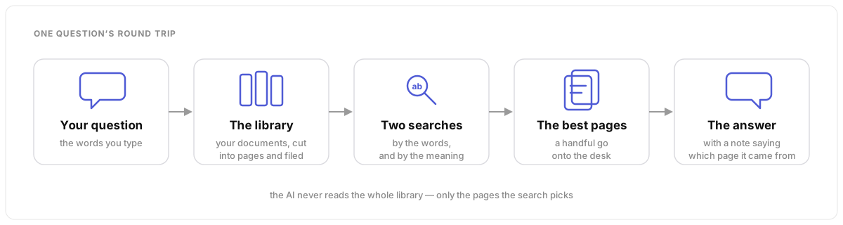
An AI only knows what it learned in school and what is on its desk. To answer questions about your documents, something has to find the right pages first. That something is retrieval: two kinds of librarian, a filing system built for meaning, a fair way to merge their lists, and a loop that turns it all into a chat.
The whole trip in one picture
Open book, not closed book
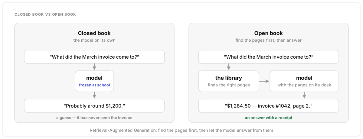
The model’s knowledge stopped the day its training ended, and it has never seen your files. Ask it what the March invoice came to and it will guess, politely and confidently. So we change the exam. Find the right pages first, put them on the desk next to the question, and let the model answer from what is in front of it. That is all RAG is: retrieve, then generate. The desk is small, so the finding has to be good.
Under the hood
Retrieval-augmented generation (Lewis et al., 2020): retrieve the top-k passages for a query, place them in the prompt alongside the question, and generate. It addresses the knowledge cut-off, private data and freshness without fine-tuning, makes citations possible, and reduces (but does not eliminate) fabrication. The ceiling is the retriever: if the right passage is not on the desk, the model cannot answer from it, and a wrong passage produces a confident wrong answer. Retrieval quality is measured separately from answer quality, as recall at k.
Cut into pages, filed twice
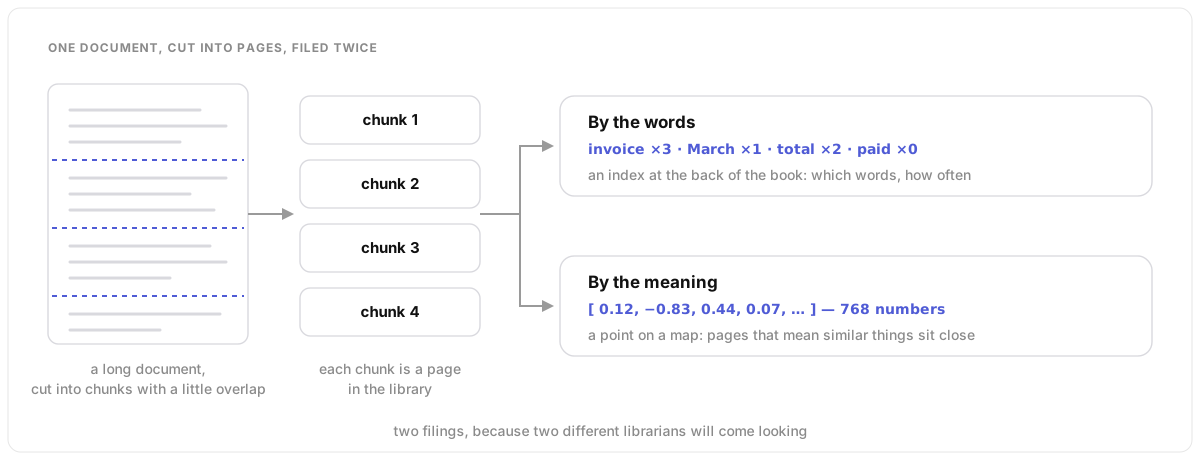
A whole document is too big to search well as one lump, so it is cut into chunks: a few paragraphs each, with a little overlap so nothing is sliced mid-thought. Each chunk is then filed two ways. Once by the words it contains, the way an index at the back of a book works. And once by what it means, as a point on a map. Two filings, because two very different librarians will come looking.
Under the hood
Chunking strategies: fixed token windows with overlap, splits on headings and structure, or semantic splits. Size is a trade-off: small chunks are precise but lose surrounding context, large chunks dilute the signal and crowd the context window. Each chunk carries metadata (source document, page, date, client, type) so results can be filtered and cited. Both the inverted index for keyword search and the embedding for vector search are computed once at ingest, which is what makes search cheap at query time.
The librarian who counts words
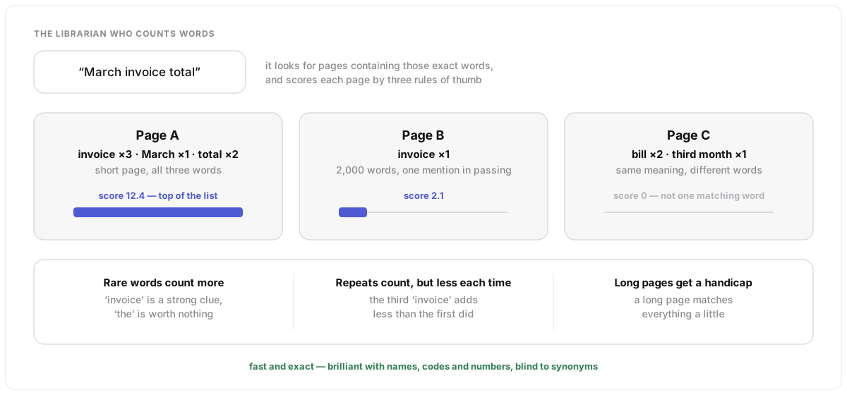
The first librarian reads only the words. Ask for “March invoice total” and it finds pages containing those exact words, scored by three rules of thumb. Rare words count more: “invoice” is a strong clue, “the” is worthless. Repeats count, but less each time. And long pages get a handicap, because a long page matches everything a little. It is fast, exact, and brilliant with names, codes and numbers. But “bill” and “invoice” are strangers to it.
Under the hood
This is BM25 (“Best Match 25”), the classic ranking
function from the probabilistic relevance framework (Robertson &
Zaragoza). For each query term it multiplies an inverse document
frequency (rarer across the corpus means higher weight) by a saturating
term-frequency term, tf·(k1+1) / (tf + k1·(1 −
b + b·|d|/avgdl)), where k1 (about 1.2 to
2) controls how quickly repeats stop helping and b (about
0.75) controls the length normalisation. It runs over an inverted
index, word to list of chunks, needs no model, and is hard to beat on
identifiers, product codes, exact phrases and numbers. It is purely
lexical: stemming and tokenisation help at the edges, but synonyms are
invisible to it.
The librarian who understands meaning
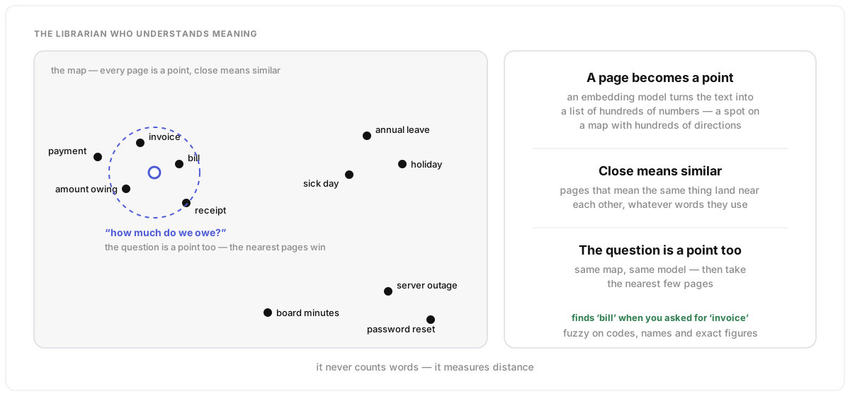
The second librarian never counts a word. An embedding model turns each page into a long list of numbers, which is really a point on a map with hundreds of directions. Pages that mean similar things land close together: “invoice”, “bill” and “amount owing” are neighbours, and “annual leave” is far away. Your question becomes a point on the same map, and the nearest pages win. This finds “bill” when you asked for “invoice”. But it is fuzzy on exactly what the first librarian is good at: codes, names and exact figures.
Under the hood
Embeddings are dense vectors (typically a few hundred to a few thousand dimensions) produced by a model trained so that semantically similar text lands close together. Similarity is cosine or dot product; retrieval is k-nearest-neighbours. The query must be embedded with the same model as the corpus, and changing the model means re-embedding everything. Strengths: paraphrase, synonyms, and often cross-lingual matching. Weaknesses: exact-match terms, numbers, rare identifiers and domain jargon the embedding model never saw. The embedding model is a separate, much smaller model from the chat model, and it is cheap to run.
A filing system for points
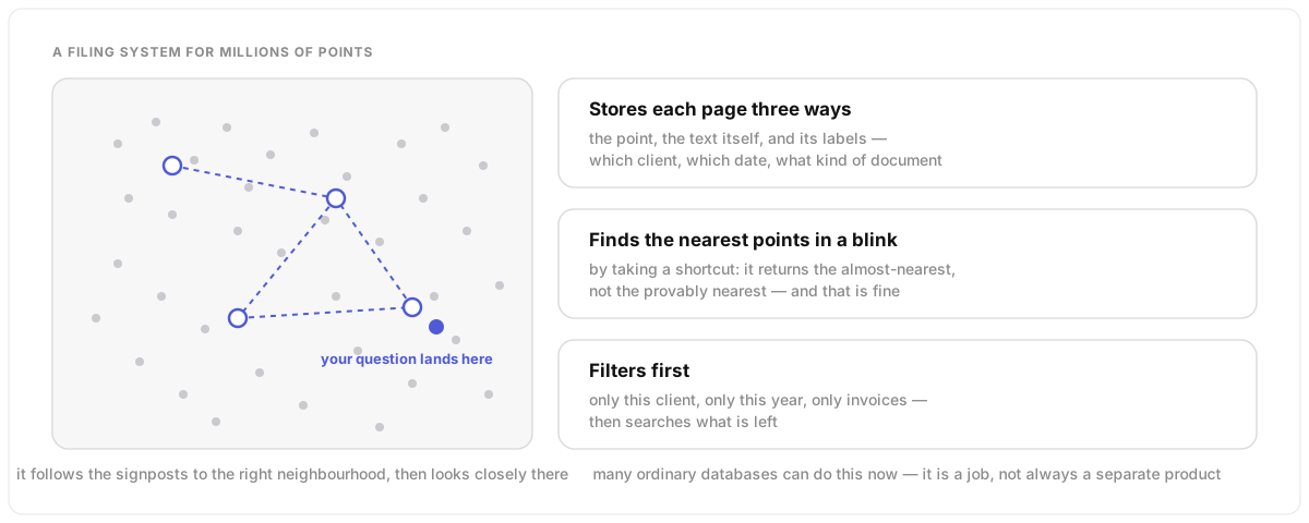
Millions of points on a map, and you need the nearest few in a blink. A vector database is built for exactly that. It stores each page’s point alongside the text itself and its labels: which client, which date, what kind of document. It finds near neighbours fast by taking a shortcut: instead of measuring every point, it follows signposts to the right neighbourhood and looks closely there, so it returns the almost-nearest rather than the provably nearest. And it can filter first: only this client, only this year. Many ordinary databases can do this now, so it is a job, not always a separate product.
Under the hood
Approximate nearest-neighbour indexes (HNSW graphs, IVF partitions,
product quantisation) trade a little recall for orders of magnitude in
speed; parameters such as ef_search or nprobe
tune recall against latency. Options range from extensions to a
database you already run (Postgres with pgvector, SQLite, Elasticsearch
and OpenSearch) to dedicated stores (Qdrant, Weaviate, Milvus,
Pinecone), and most now ship BM25 too, so one store can serve both
searches. Metadata filtering matters for multi-tenant data, and
pre-filtering versus post-filtering affects both speed and recall.
Store the chunk text and its provenance with the vector, or the answer
cannot cite anything.
Two lists into one
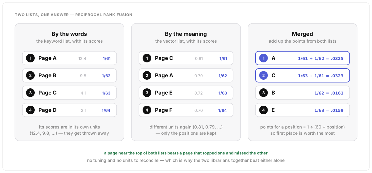
Now you have two ranked lists from two librarians who score things in completely different units. Reciprocal Rank Fusion throws the scores away and keeps only the positions. Every page gets points for where it sits on each list: first place is worth the most, second a little less, and so on down. Add up the points. A page near the top of both lists beats a page that topped one and missed the other. No tuning, no units to reconcile, and it is why the two librarians together beat either one alone.
Under the hood
Reciprocal Rank Fusion (Cormack, Clarke & Büttcher, 2009):
score(d) = Σ 1 / (k + rank_i(d)) across the lists
that contain d, with k usually 60. Because it is
rank-based it needs no score normalisation, which is exactly the
problem with combining a BM25 score and a cosine similarity directly.
Alternatives are weighted score fusion after min-max normalisation, or
a cross-encoder reranker run over the union of the top candidates:
slower and more accurate, often used as a final pass over the top 20
to 50. Hybrid retrieval is the production default because BM25 catches
identifiers and exact phrases while vectors catch paraphrase.
Putting it into a chat
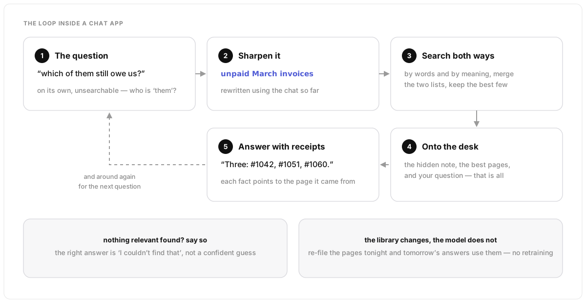
Here is the loop inside a real chat app. You ask, “which of them still owe us?”. On its own that is unsearchable, so the app first sharpens it using the conversation so far: “unpaid March invoices”. Both librarians search, the lists are merged, and the best handful of pages go onto the desk next to your question and the hidden note. The model answers from those pages and says which page each fact came from. If nothing relevant turns up, the right answer is “I couldn’t find that”, not a confident guess. And when the documents change, you re-file the pages; the model itself never changes.
Under the hood
The pipeline: condense the question with chat history (or generate a hypothetical answer to embed), hybrid retrieval, RRF, an optional reranker, then the top few chunks (often 5 to 10) into the prompt with source ids. The system prompt instructs the model to answer only from the supplied context, cite by id, and say when the context does not contain the answer. Common failures: the retriever misses (nothing relevant on the desk), too many chunks and the model gets lost in the middle, a stale index, or a chunk boundary that cuts the answer in half. Freshness comes from re-indexing, never retraining. In agent setups the search is simply a tool the model calls for itself, as many times as it needs.